Blaschke Tool User's Guide
Back to Applet
Introduction
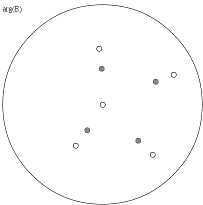 To get started with the applet, first specify the zeroes of the Blaschke
product that you want to investigate. Each white circle is a zero of the Blaschke product, and the grey circles are drawn
at the critical points. The white points (except for the zero at zero) can be dragged around the circle. Double-clicking
on the circle will add a new zero at that point, and dragging a zero outside of the circle will remove it. The grey critical
points will be automatically recomputed. Numerical values for the Zeroes, Critical Values, and Critical Points are displayed
to the right of the circle.
To get started with the applet, first specify the zeroes of the Blaschke
product that you want to investigate. Each white circle is a zero of the Blaschke product, and the grey circles are drawn
at the critical points. The white points (except for the zero at zero) can be dragged around the circle. Double-clicking
on the circle will add a new zero at that point, and dragging a zero outside of the circle will remove it. The grey critical
points will be automatically recomputed. Numerical values for the Zeroes, Critical Values, and Critical Points are displayed
to the right of the circle.
One can also enter the zeroes of a Blaschke product in the "Load/Edit" box, and click Load to configure the Blaschke product to use those zeroes. Clicking "Permalink" will generate a web link with these zeroes
which can be bookmarked for future reference.
Tip: if you want to see a Blaschke product without a zero at zero, you can remove it from the "Load/Edit" box and click
Load.
N.B. Blaschke products can have a leading term of modulus 1. The applet uses a Blaschke product of the form
 . Another useful form is to write the numerator of each term as (ai-z) and keep the same denominator. Single-factor Blaschke products of that form have the benefit of being self-inverse.
Plots
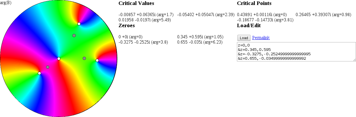
 The user can generate or regenerate a color
plot the argument of the Blaschke product by clicking the Plot button. This generates three
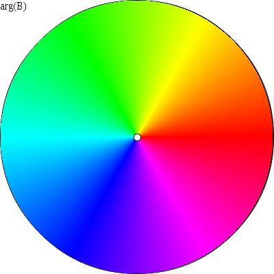
plots: "arg(B)," "Region Preimages," and "Region Images." Each color on the "arg(B)" plot corresponds to an angle λ
For example:
The user can generate or regenerate a color
plot the argument of the Blaschke product by clicking the Plot button. This generates three
plots: "arg(B)," "Region Preimages," and "Region Images." Each color on the "arg(B)" plot corresponds to an angle λ
For example:
- Red: B(z) is real
- Green: B(z) = r*ei(2/3)π
- Blue: B(z) = r*ei(4/3)π
Region Preimages and Region Images
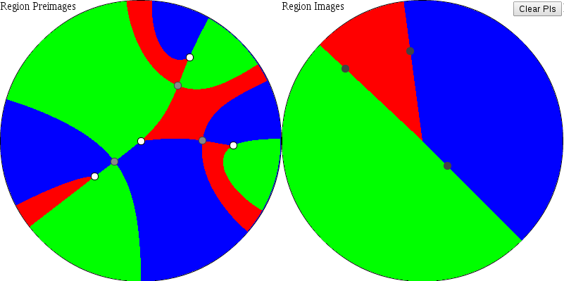
The Region Images plot divides the circle into regions bounded by curves which pass through the critical points of the
plot. (Each curve is a preimage of f(t) = t * ei*arg(w) where w is a critical value of B.) In the illustration
below, each region on the left of a given color maps one-to-one with to the region of the same color on the right. The
grey circles in the "Region Images" plot are the critical values of the Blaschke product (which lie on the boundaries
between the colored regions. Also observe that in this example there are four regions of each color on the left hand
side (one adjacent to each zero), illustrating the fact that a Blaschke product of degree n is an n-to-1 map.
Plotting Preimages
Clicking in the "Region Images" circle and dragging one's mouse around will draw, in the "Region Preimages" circle, the
points which map to the points which you drag over. Clicking the Clear PIs button clears
those paths.
Find Preimages
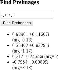 The Find Preimages utility lets you enter
an imaginary number in
The Find Preimages utility lets you enter
an imaginary number in
x+yi
format, and it will find points which map to that value under the Blaschke product.
Drawing lines
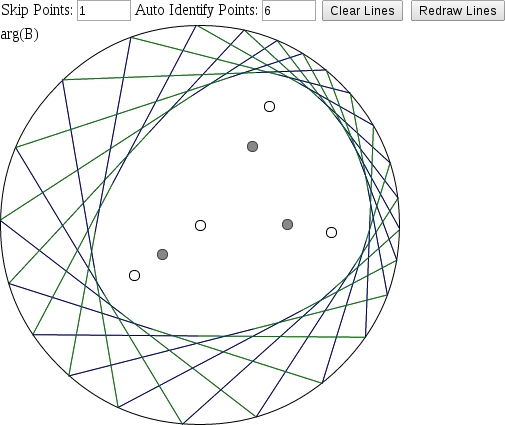 The applet can also draw lines which help to illustrate the
properties of the Blaschke-Poncelet curves. Entering a value N in the "Auto Identify Points" box will pick N for λ
and the applet will then plot lines connecting the points which B maps to eiλ. Entering a value M other
than 1 in the "Skip Points" box will instead skip M points when drawing lines.
The applet can also draw lines which help to illustrate the
properties of the Blaschke-Poncelet curves. Entering a value N in the "Auto Identify Points" box will pick N for λ
and the applet will then plot lines connecting the points which B maps to eiλ. Entering a value M other
than 1 in the "Skip Points" box will instead skip M points when drawing lines.
Options
The "Auto Re-Draw" checkbox will automatically replot these lines as the zeroes of the Blaschke product are manipulated.
The "Guess Ellipse" checkbox will attempt to fit an ellipse to that curve. The "Solid Lines" checkbox will draw the approximation
to the Poncelet curve in red, and draw the ellipse (if specified) with bolder lines.
Acknowledgements
This code uses the Numeric.js numerics library for javascript, jQuery.
The algorithm to best-fit an ellipse to a set of data points was adapted from a Python example Fitting an Ellipse to a Set of Data Points.